Calculate a spatial gradient

Here is a small demo I made to answer a collegue’s question: how would you calculate a spatial gradient (for example of a temperature \(T(x,y)\)) in R, given the formula:

\[ \vec{\nabla T}(x,y) \simeq \{ \frac{T(x+1,y) - T(x-1,y)}{2dx};\frac{T(x,y+1) - T(x,y-1)}{2dy} \} \]

I will use for this small demo data.table for the data manipulations and ggplot2 for plots. I will show at the end how do the same with dplyr.

library(data.table)
library(ggplot2)
library(dplyr)

## 
## Attachement du package : 'dplyr'

## The following objects are masked from 'package:data.table':
## 
##     between, first, last

## The following objects are masked from 'package:stats':
## 
##     filter, lag

## The following objects are masked from 'package:base':
## 
##     intersect, setdiff, setequal, union

As an example, I create first a guassian field, on which I will try to calculate the gradient. I create it as a data.frame, in the long format, for a given (space) size:

size <- 100

field <- data.table( x = rep(seq(-size/2,size/2,1),size+1), y = rep(seq(-size/2,size/2,1),each = size+1))
field$temp <-  exp(-(field$x^2 + field$y^2)/(size^2))
head(field)

##      x   y      temp
## 1: -50 -50 0.6065307
## 2: -49 -50 0.6125651
## 3: -48 -50 0.6185359
## 4: -47 -50 0.6244400
## 5: -46 -50 0.6302744
## 6: -45 -50 0.6360361

The usual would be to have a matrix, with the row indicating the x position and thecolumns indicating the y. You can transform from long to wide with reshape or with melt and dcast from data.table.

matrix_field <- dcast(x~y,value.var = "temp",data = field)
head(matrix_field[,1:5])

##      x       -50       -49       -48       -47
## 1: -50 0.6065307 0.6125651 0.6185359 0.6244400
## 2: -49 0.6125651 0.6186596 0.6246898 0.6306527
## 3: -48 0.6185359 0.6246898 0.6307788 0.6367998
## 4: -47 0.6244400 0.6306527 0.6367998 0.6428782
## 5: -46 0.6302744 0.6365451 0.6427496 0.6488849
## 6: -45 0.6360361 0.6423641 0.6486254 0.6548167

You can pass (re-pass) to long format with the melt function:

melt(matrix_field,id.vars = "x",variable.name = "y",value.name = "temp") %>%
  head()

##      x   y      temp
## 1: -50 -50 0.6065307
## 2: -49 -50 0.6125651
## 3: -48 -50 0.6185359
## 4: -47 -50 0.6244400
## 5: -46 -50 0.6302744
## 6: -45 -50 0.6360361

Lets plot this field with ggplot:

p <- ggplot(data = field,aes(x,y)) +
  geom_tile(aes(fill = temp))+
  scale_fill_gradient(low = "green", high = "red")+
  theme_light()+ 
  coord_fixed()
p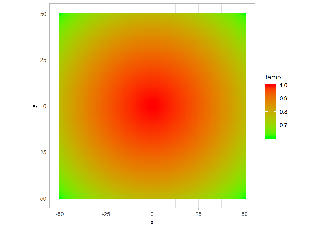

Here I use coord_fixed to have the same length on the x and y axis, as I want to see the shape of the plot.

Now to calculate the gradient, I need to make the difference between \(T(x+1)\) and \(T(x-1)\) and center it on \(x\), for all \(x\) and each fixed \(y\). The simpliest way is this one:

field[,.(x,
         `temp x+1` = c(NA,temp[3:.N],NA),
         `temp x-1` = c(NA,temp[1:(.N-2)],NA),
         `temp x` = temp)] %>%
  head()

##      x  temp x+1  temp x-1    temp x
## 1: -50        NA        NA 0.6065307
## 2: -49 0.6185359 0.6065307 0.6125651
## 3: -48 0.6244400 0.6125651 0.6185359
## 4: -47 0.6302744 0.6185359 0.6244400
## 5: -46 0.6360361 0.6244400 0.6302744
## 6: -45 0.6417221 0.6302744 0.6360361

We do that for each y value using the by grouping of data.table, and obtain the \(x\) and \(y\) components of the gradient.

gradx <- field[,.(gradx = c(NA,temp[3:.N],NA)-c(NA,temp[1:(.N-2)],NA), x = x),by = y] 
grady <- field[,.(grady = c(NA,temp[3:.N],NA)-c(NA,temp[1:(.N-2)],NA), y = y),by = x] 

We can merge them into a single data.table;

grad <- merge(gradx,grady, by = c("x","y")) 
head(grad[abs(x) < 10 & abs(y) < 10])

##     x  y       gradx       grady
## 1: -9 -9 0.003541798 0.003541798
## 2: -9 -8 0.003547824 0.003153621
## 3: -9 -7 0.003553149 0.002763560
## 4: -9 -6 0.003557772 0.002371847
## 5: -9 -5 0.003561687 0.001978714
## 6: -9 -4 0.003564894 0.001584397

I want to represent the gradient on my first plot. I take ten values of the gradient on x and y:

gradplot <- grad[x %in% seq(-size,size,round(size/10)) & y %in% seq(-size,size,round(size/10))] 

and then add the arrows with directions and norms proportional to the calculated gradient to the first plot:

p + 
  geom_segment(data = gradplot,
               aes(x,y,xend =x+ gradx*500,yend =  y+grady*500), 
               arrow = arrow(length = unit(0.01,"npc"))) 

## Warning: Removed 40 rows containing missing values (geom_segment).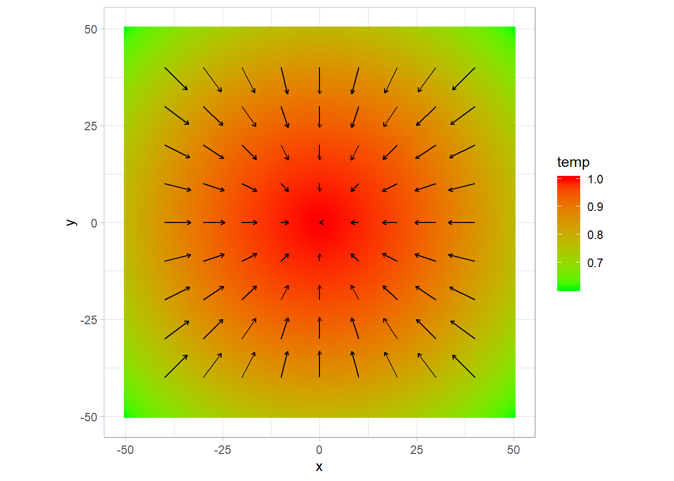

The same calculation with dplyr:

gradx <- field %>% # gradient selon x
  group_by(y) %>%
  mutate(gradx = c(NA,temp[3:n()],NA)-c(NA,temp[1:(n()-2)],NA))
grady <- field %>% # gradient selon y + merge
  group_by(x) %>%
  mutate(grady = c(NA,temp[3:n()],NA)-c(NA,temp[1:(n()-2)],NA)) 

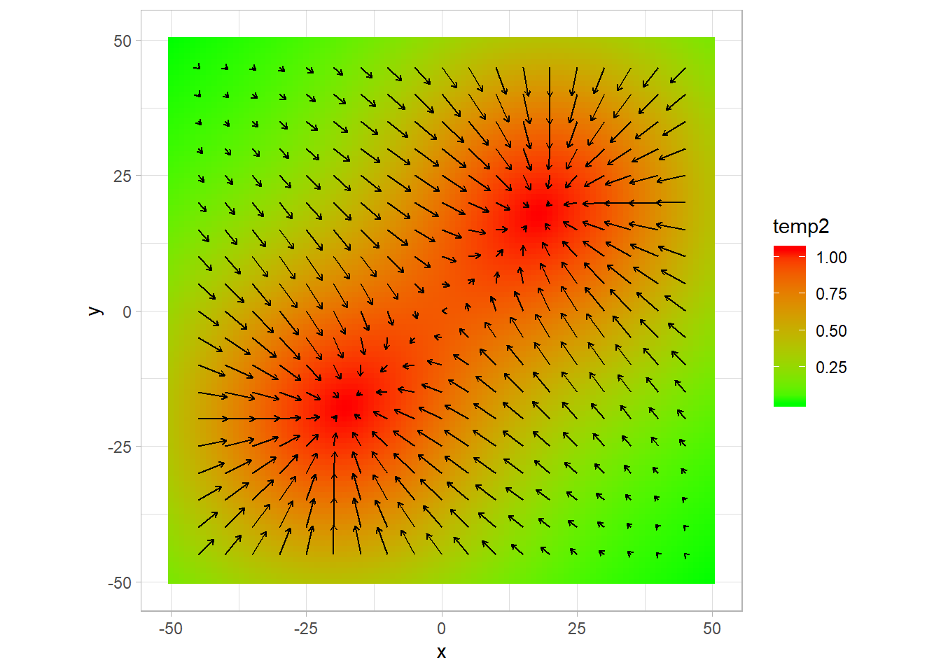
grad <- full_join(gradx,grady, by = c("x","y"))

For a more complex pattern, you can do the same.

field[,temp2 :=  exp(-( (x - 20)^2 + (y - 20)^2)/(size^2/10)) + exp(-( (x + 20)^2 + (y + 20)^2)/(size^2/10))]
p2 <- ggplot(data = field,aes(x,y)) +
  geom_tile(aes(fill = temp2))+
  scale_fill_gradient(low = "green", high = "red")+
  theme_light()+ 
  coord_fixed()

gradx <- field[,.(gradx = c(NA,temp2[3:.N],NA)-c(NA,temp2[1:(.N-2)],NA), x = x),by = y] 
grady <- field[,.(grady = c(NA,temp2[3:.N],NA)-c(NA,temp2[1:(.N-2)],NA), y = y),by = x] 
grad <- merge(gradx,grady, by = c("x","y")) 
gradplot <- grad[x %in% seq(-size,size,round(size/20)) & y %in% seq(-size,size,round(size/20))] 
p2 + 
  geom_segment(data = gradplot,
               aes(x,y,xend =x+ gradx*100,yend =  y+grady*100), 
               arrow = arrow(length = unit(0.01,"npc"))) 

## Warning: Removed 80 rows containing missing values (geom_segment).