outline
- R: what is it for ?
- R: base syntax
- R: the packages you need to know/learn to be efficient
- Demos on physicists data
- The pitfalls to avoid
- how to learn and where to look
R is created in 1995
An open source implementation of S (Bell labs statistical software)
Designed to make data analysis and statistics easy
interpreted language, high level
Primarily used in academics, moving to enterprise lately
Pros
- open source, so free
- Wonderful IDE: Rstudio
- variable exploration
- help, plot tools
- github integrated
- huge community! so lot of helps

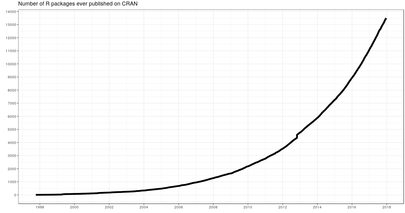
- Lots of tools (libraries)
- easy to paralelize, can be used on baobab

Cons
- Slow (not for Whab or Nico, but some library are coded in C)
- lots of ways to do the same things, so a bit messy in the beginning
- hard to find the appropriates tools in the beginning (but i ll give you the good ones)
- steep learning curve, but accesible for experienced programmers or physicists
Basic syntax
When you install R, it comes with base package and 6 others.
R is interpreted, and guess the type you declare (like matlab and python)
a <- 2
b = 2
a
b
data type
a <- "plouf"
class(a)
b <- 2
class(b)
c <- 2L
class(c)
d <- as.factor("plouf")
class(d)
WTF factor ?
a
d
as.numeric(a)
as.numeric(d)
used in statistical model (generalised linear models, etc), but dangerous
data structure type
vector
# vector
a <- c(2,5,7,8)
a
class(a)
a[1]
a[1:2]
a[1,4]
a[c(1,4)]
everything same class, so coerce things
a <- c(2,5,7,"plouf")
class(a)
a[1]
matrix
b <- matrix(c(3,4,5,8),nrow = 2, ncol = 2)
b
b[1,]
b[,2]
b[1]
all matrix operation exists, equation solving etc.
list
c <- list(trucs = c(1,5,7), plouf = "des choses", matrice = matrix(sample(1:100,25),5,5) )
c
c$trucs
c[[1]]
c[["trucs"]]
c["trucs"]
data frame: une liste avec contrainte de dimension !
C'est le coeur du traitement de données dans R
d <- data.frame(experiment = rep(LETTERS[1:5], each = 2), data1 = sample(c(0,1),10,replace = T), data2 = sample(1:100,10))
d
#idem list:
d$experiment
d[,"experiment"]
d$experiment[1]
d[1,"experiment"]
d[1,1]
Esay to subset using boolean.
d$experiment
d$experiment == "A"
d[d$experiment == "A",]
loops and conditional
d[d$data2 > 50 & d$data1 == 0,]
d[d$data2 > 50 | d$data1 == 0,]
for(i in 1:4){
    if(i>2){
        print(paste0(i," est sup à 2" ))}else{
        print(paste0(i," est inf à 2" ))}
}
Specific of R, really usefull: lapply and sapply (and others)
plouf <- lapply(1:4,function(x){x^2})
plouf
class(plouf)

plouf2 <- sapply(1:4,function(x){x^2})
plouf2
class(plouf2)
sapply(c("data1","data2"),function(col){
    summary(d[,col])
})
Libraries
library(ggplot2) # pour les graphiques
head(mpg)
ggplot(data = mpg) +
  geom_point(aes(x = displ, y = hwy, color = class))

ggplot(data = mpg) +
  geom_point(aes(x = displ, y = hwy)) +
  facet_grid(drv ~ cyl)

library(data.table) # pour le data management
dt <- setDT(copy(mpg))
class(dt)
plus <- data.table(manufacturer = c('audi','chevrolet','dodge','ford','honda','hyundai','jeep','land rover','lincoln','mercury','nissan','pontiac','subaru','toyota','volkswagen'),
                   country = c("DE","US","US","US","JP","JP","US","UK","UK","US","JP","US","DE","JP","DE"))
head(plus)
merged <- merge(dt,plus,on = "manufacturer")
head(merged)
merged[country == "DE",.(mean_comsum = mean(hwy)),by = .(manufacturer,model)]
You would have made a double loop with condition. With 10 000 000 rows, 100000 groups you can't. Here it is efficient and concise. Alternative :
library(dplyr) # more or less equal perf
library(stringr) # to deal efficiently with strings
dose <- c("20 g/kg", "30g/kg lkd","15000 mg/kg")
dose
dose_corr <- data.frame( unit1 = str_extract(dose,"[a-z]+(?=/)"),
                  unit2 = str_extract(dose,"(?<=/)[a-z]+"),
                  value = str_extract(dose,"[0-9]+"))
dose_corr
library(lmerTest)
library(lme4)
regressions linéaires, non linéaires, multiniveau, lineaire généralisé etc
a1_mean = 3
b1_mean = 0
curves <- data.table( curve = rep(letters[1:5],each = 10),
                     time = rep(1:10,5),
                     a1 = rep(rnorm(5,a1_mean,1),each = 10),
                     b1 = rep(rnorm(5,b1_mean,1),each = 10))

curves[, y_data := a1*time + b1 + rnorm(.N,0,2), by = curve]
curves[, y_real := a1*time + b1 , by = curve]
Create 5 curves with slope normaly distrib around a1_mean and intercept around b1_mean, with a bit of noise.
p <- ggplot(data = curves )+
geom_point(aes(time,y_data,color = curve),size = 3)+
geom_line(aes(time,y_real,color= curve),linetype = "dashed")+
theme_light()
p

fit <- lmer(y_data ~ time + (1 + time|curve) , data = curves)
summary(fit)
curves[,y_fit := predict(fit, newdata = curves)]

p + geom_line(aes(time,y_fit,color= curve),linetype = "solid")

Some others
- librudate for date handling
- rshiny to generate java/html interactives pages with buttons and graphs (amazing)
- reporters to generate table directly in word
- parallel to do parallel calculation
now real physicist examples:
- the join experiment I did with PSI in 2014.
- one hour in R , weeks during my post doc and matlab.
The experiment:
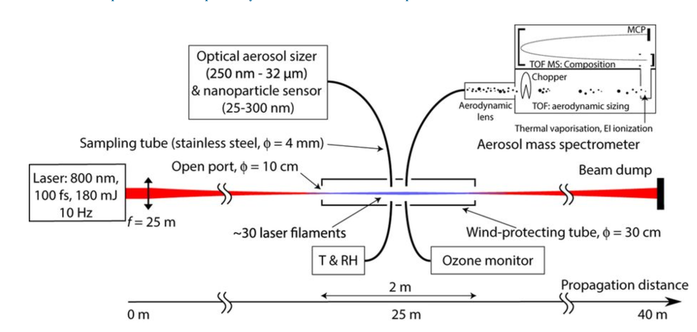
three main devices :
- arduino, say if laser is on or off
- grimm for particles sizes
- AMS, for composition (and size)
library(ggplot2)
library(data.table)
library(stringr)
library(lubridate)
setwd("C:/Users/dmongin/Documents/presentation_R_pourlesnuls/PSI")
list.files(pattern =  ".txt$")
arduino <- fread("arduino_tot.txt")
head(arduino)
Here a stupid person didn't put any name (and its me), and didn't use any formating for the date. Here is the date formating
arduino[,Date := ymd_hms(paste0(V1,".",V2,".",V3," ",V4,":",V5,":",V6))] # make a string with all year month day and HMS
head(arduino)
arduino[,laser := V10]
arduino[,ozone := V9]
table(arduino[,.N,by = Date]$N) # table of line number per date (i.e. per second)
Multiple lines with the same exact date !! Only one measure per second and variable of interest:
arduino[,N := .N,by = Date] # N is the number of line per Date
arduino_clean <- arduino[N == 1,.(Date,laser,ozone)] # subselection
head(arduino_clean)
ggplot(data = arduino_clean,aes(Date,ozone))+ # define data, x and y
  geom_line()+ # curve type
  geom_ribbon(aes(Date,ymin = 0,ymax = laser*500),fill = "red", alpha = 0.1)+ # make area trasparent
  theme_light()+ # choose theme
  facet_wrap(~date(Date),scales = "free") # one plot per day

testo <- fread("testo_tot.txt") # read
testo[,Date := ymd_hms(paste0(V1,".",V2,".",V3," ",V4,":",V5,":",V6))]# define the date
testo[,temp := V9] # define temp column
testo[,humidity := V8]
testo_clean <- testo[,.(Date,temp,humidity)] # subselect the columns of interest
head(testo_clean)
plouf <- merge(testo,arduino_clean,all.x = T,on = "Date") # merge arduino and testo
ggplot(data = plouf)+ # plot
  geom_line(aes(Date,temp,color = "temperature"))+
  geom_line(aes(Date,humidity,color = "humidity"))+
  geom_ribbon(aes(Date,ymin = 0,ymax = laser*100,fill = "laser"), alpha = 0.2)+
  theme_light()+  facet_wrap(~date(Date),scales = "free")

summary(lm(ozone ~ laser + humidity,data = plouf))
summary(lm(humidity ~ laser + temp,data = plouf))
grim <- fread("grimm_tot.txt") # read file
setnames(grim,"[d&t31.12.2035 11:50:55]","date") # change weird name
grim[,Date := dmy_hms(date)] # make date
grim[,N := .N,by = Date] # count the number of line per date
grim <- grim[N == 1] # select just one line per s
head(grim)
I switch to long format instead of broad:
grim_clean <- melt(grim,measure.vars = patterns("m$"),variable.name = "size",value.name = "concentration")
head(grim_clean)
I change the size to numbers
grim_clean[,size := as.numeric(str_extract(size,"[0-9]+\\.[0-9]+"))] # extract just numbers of size
grim_clean <- grim_clean[,.(Date,size,concentration)]
head(grim_clean)
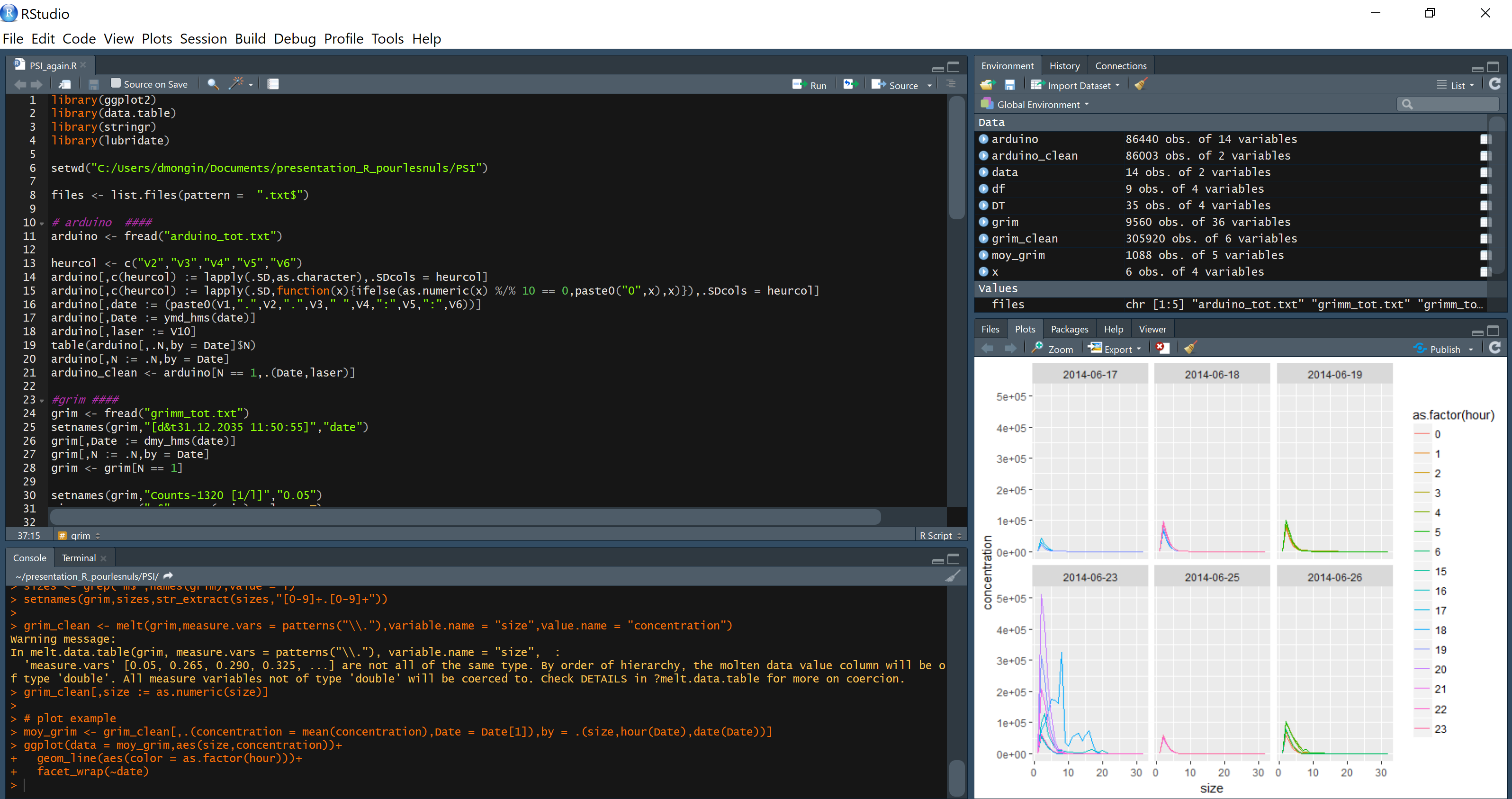
Example : plot the mean concentration per hour, for each day of the experiment:
moy_grim <- grim_clean[,.(concentration_m = mean(concentration)),by = .(size,hour(Date),date(Date))]
head(moy_grim)
ggplot(data = moy_grim,aes(as.numeric(size),concentration_m))+
  geom_line(aes(color = as.factor(hour),group = hour))+
  facet_wrap(~date,scales = "free")+ theme_light() +
  scale_y_log10() +
  labs(x = "size um", y = "concentration", color = "day hour")

AMS <- fread("timeserie_ams4.txt")
AMS[,Date := dmy_hms(time_stamp)]
head(AMS)
define three experiment (dont remember):
# define 3 experiment with the dates
exp1 <- ymd(c("2014-06-17","2014-06-18","2014-06-19"))
exp2 <- ymd(c("2014-06-23"))
exp3 <- ymd(c("2014-06-25","2014-06-26"))

# for the date in each group, define new variable exp
grim_clean[date(Date) %in% exp1,exp := "exp1"]
grim_clean[date(Date) %in% exp2,exp := "exp2"]
grim_clean[date(Date) %in% exp3,exp := "exp3"]

AMS[date(Date) %in% exp1,exp := "exp1"]
AMS[date(Date) %in% exp2,exp := "exp2"]
AMS[date(Date) %in% exp3,exp := "exp3"]
I merge arduino results and AMS to have the laser
plouf <- merge(arduino_clean,AMS,all.y = T,by = "Date")
plouf <- plouf[!is.na(laser)]
head(plouf)
change to long format
AMS_long <- melt(plouf,measure.vars = c("Tot","Org","SO4","NO3","NH4","Chl","Org43","Org44"),value.name = "concentration",variable.name = "type")
head(AMS_long)
# calculate the mean per aerosol type, laser state and experiment
result_AMS <- AMS_long[type != "Tot",.(concentration_m = mean(concentration)),by = .(laser,type,exp)]
# do the plot
ggplot(data = result_AMS,aes( as.factor(laser) ,concentration_m,fill = type))+
  geom_col()+
  facet_wrap(~ exp, scales = "free")+
  labs( x = "laser", y = "concentration ppm", color = "type", fill = "type" ) + theme_light()

To visualize the time serie in time: not complicated either
ggplot(data = AMS_long[,laser_n := laser*max(concentration),by = exp],aes(Date,concentration))+
  geom_ribbon(aes(Date,ymin = 0,ymax = laser_n),fill = "red", alpha = 0.1)+
  geom_line(aes(colour = type))+ facet_wrap(~exp,scales = "free")+ theme_light()

Pitfalls
don't re-descover, use the libraries
use long format, grouping operation, and ggplot to make your life easy.
- Long format : each column a variable.
- Example grimm: All columns are particles concentration -> two columns, one concentration, the other size
spending time on data management makes life easier after. So:
- check if your unique values are unique
- always look out for missing values
- define the column type when importing data: make numeric variable numeric, avoid factors
Ressources
- http://r4ds.had.co.nz/ : R for Data science. Author is head of Rstudio, inventor of ggplot, dplyr, libridate, Rshiny etc. Ressource free online.
- stackoverflow ! Carefull:
- Check if the question is already asked
- Give a reproducible small example of your problem, so people can give solution(s)
- Be specific, show that you tried something
- If so, 20 minutes to have an answer max
- Rlunchs at unige ! http://use-r-carlvogt.github.io/prochains-lunchs/
Proof of warming in geneva in 20 lines of R
setwd("C:/Users/dmongin/Documents/presentation_R_pourlesnuls")
Geneva <- read.csv("test.txt",sep = ";",skip = 27)
head(Geneva)
Geneva <- setDT(Geneva)
Geneva[,dec := Year %/% 10]
Geneva[,Temperature_dec := mean(Temperature),by = .(dec,Month)]

ggplot(data = Geneva,aes(Month,Temperature_dec))+
  geom_line(aes(color = as.factor(dec*10)))+
  theme_light()+
  labs(  color = "decennie", title = "mean per decennie",  y = "Temperature",   x = "Months"  )
options(repr.plot.width=8, repr.plot.height=4.5)

library(zoo)

nyear <- 5
Geneva[,Temperature_rollmean := c(rollmean(Temperature,nyear,align = "center",fill = NA)), by = Month]
fit <- lmer(Temperature ~ I(Year/100) + (1+I(Year/100)|Month),data = Geneva)
Geneva[,Temperature_predict := predict(fit,newdata = Geneva)]
summary(fit)
ggplot(data = Geneva)+
  geom_point(aes(Year,Temperature_rollmean,color = as.factor(Month)))+
  geom_line(aes(Year,Temperature_predict,color = as.factor(Month)))+
  theme_light()+
  labs(   color = "Month",  title = "Evolution",   y = "Temperature",    x = "Year"  )

calculation of gradient
taille <- 100
field <- data.table( x = rep(seq(-taille,taille,1),2*taille+1), y = rep(seq(-taille,taille,1),each = 2*taille+1))
field[,temp := exp(-(x^2 + y^2)/10000)]
p <- ggplot(data = field,aes(x,y)) +
  geom_tile(aes(fill = temp))+
  scale_fill_gradient(low = "green", high = "red")
p

gradx <- field[,.(gradx = c(NA,temp[3:.N],NA)-c(NA,temp[1:(.N-2)],NA), x = x),by = y] #gradient selon x
grady <- field[,.(grady = c(NA,temp[3:.N],NA)-c(NA,temp[1:(.N-2)],NA), y = y),by = x] # gradient selon y
grad <- merge(gradx,grady, by = c("x","y")) # merge des deux

# je prend 10 fleche par lignes, sinon y en a trop.
gradplot <- grad[x %in% seq(-taille,taille,round(taille/10)) & y %in% seq(-taille,taille,round(taille/10))]
# je renormalise le gradient pour que la longueur des fleches soit appreciable sur le plot
gradplot[,c("gradx","grady"):= .(gradx/max(gradx,na.rm = T)*10,grady/max(grady,na.rm = T)*10)]
p + geom_segment(data = gradplot,aes(x,y,xend =x+ gradx,yend = y+grady), arrow = arrow(length = unit(0.2,"cm")))
