COVID19 data: pdf scrapping
getting data
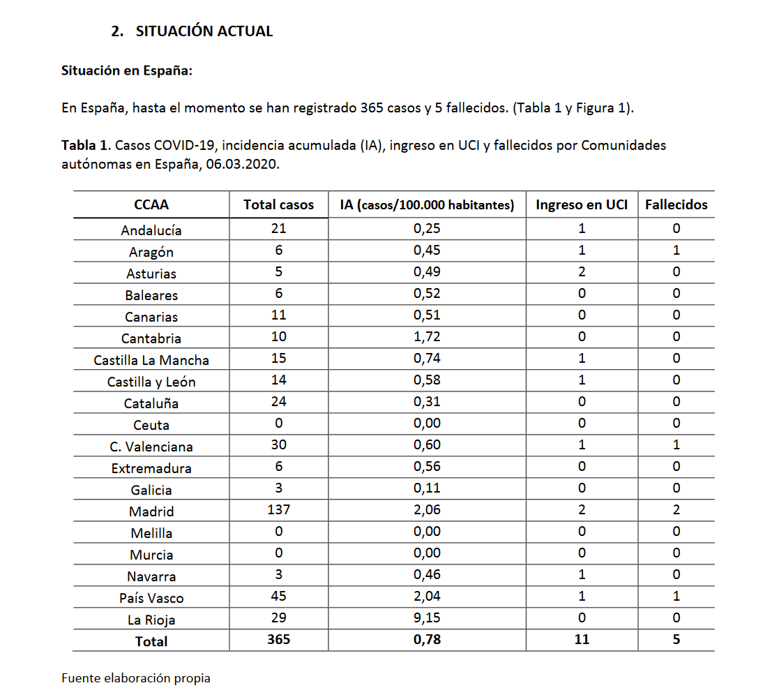
Since the COVID19 epidemic, a lot of data is published by state agency as pdf reports. For someone interested in data analysis, it is important to be able to extract these data out of the report. This is an example with COVID data in Spain given by the ministerio de sanidad. This are data by region.
Find the data
The first thing is to find one pdf report containing a report. Here is one I found, after a bit of searching, from the ministerio de sanidad page.
I contains the table I want to extract:
From the html address of the first link, you can try to guess the html address of the others, to automatize the pdf download. Here, the address https://www.mscbs.gob.es/profesionales/saludPublica/ccayes/alertasActual/nCov-China/documentos/Actualizacion_35_COVID-19.pdf" contains the report 35. You could guess all reports can be accessed just changing the number 35 in the address.
Download the data
I don’t know what is the maximum report number, and I am not sure all reports are located on the same address format. A good way to try is to use the function download.file in a loop, with a tryCatch to avoid interrupting on the first error. To download such data in R, you can do the following:
filelist <- list.files(pattern = "report[0-9]+\\.pdf")
for(i in 1:100){
  if( ! paste0("report",i,".pdf") %in% filelist){
      tryCatch(download.file(paste0("https://www.mscbs.gob.es/profesionales/saludPublica/ccayes/alertasActual/nCov-China/documentos/Actualizacion_",i,"_COVID-19.pdf"),
                destfile = paste0("report",i,".pdf"),mode = "wb"),error = function(e) e)
  }
}
Notice you need to specify the mode = "wb" in the download.file function to have readable pdf documents.
By checking the output (not shown here) you will now which pdf you managed to download or not. Here I managed to download the reports from 31 to 75, with 44 and 45 missing. Checking the report 75, It correspond to the last one, so I know the upper limit (I could have checked there). Doing some Google research with the URL name but index under 31, you will find that the first reports where under a slightly different html (and country specific) address: https://www.mscbs.gob.es/profesionales/saludPublica/ccayes/alertasActual/nCov-China/documentos/Actualizacion_“,i,”_COVID-19_China.pdf
So knowing that, this should get the rest the first reports:
filelist <- list.files(pattern = "report[0-9]+\\.pdf")
for(i in 1:31){
  if( ! paste0("report",i,".pdf") %in% filelist){
      invisible(tryCatch(
        download.file(paste0("https://www.mscbs.gob.es/profesionales/saludPublica/ccayes/alertasActual/nCov-China/documentos/Actualizacion_",i,"_COVID-19_China.pdf"),
                destfile = paste0("report",i,".pdf"),mode = "wb"),error = function(e) e))
  }
}Extract the tables
library(tabulizer)## Warning: le package 'tabulizer' a été compilé avec la version R 3.6.3library(lubridate)
library(data.table)
library(dplyr)
library(magrittr)
library(stringr)Let’s see how we can extract the tables from a pdf with tabulizer. I will try with the report 36:
out <- extract_tables(paste0("report",36,".pdf"),encoding = "UTF-8")
out
## [[1]]
## [,1] [,2] [,3] [,4] [,5]
## [1,] "" "" "" "" ""
## [2,] "" "Global" "China" "Italia" "Irán"
## [3,] "" "" "" "" ""
## [4,] "no casos" "93.062" "80.422" "2.502" "2.336"
## [5,] "IA últimos 14 días (casos" "" "" "" ""
## [6,] "" "" "0,43" "4,13" "2,88"
## [7,] "100.000 habitantes)" "" "" "" ""
## [8,] "no nuevos casos (desde última" "" "" "" ""
## [9,] "" "2.150" "119" "466" "0"
## [10,] "actualización 4/3/20 18:00)" "" "" "" ""
## [11,] "" "3.198" "2.984" "80" "77"
## [12,] "no fallecidos (L)" "" "" "" ""
## [13,] "" "(3,4)" "(3,7)" "(3,2)" "(3,3)"
## [,6] [,7] [,8] [,9]
## [1,] "Corea del" "" "" ""
## [2,] "" "Francia" "Alemania" "España"
## [3,] "Sur" "" "" ""
## [4,] "5.325" "212" "196" "198"
## [5,] "" "" "" ""
## [6,] "10,29" "0,30" "0,22" "0,38"
## [7,] "" "" "" ""
## [8,] "" "" "" ""
## [9,] "513" "8" "8" "47"
## [10,] "" "" "" ""
## [11,] "32" "4" "" "1"
## [12,] "" "" "0" ""
## [13,] "(0,6)" "(1,9)" "" "(0,6)"
##
## [[2]]
## [,1] [,2] [,3]
## [1,] "CCAA" "Total casos" "IA (casos/100.000 habitantes)"
## [2,] "Andalucía" "13" "0,15"
## [3,] "Aragón" "0" "0,00"
## [4,] "Asturias" "2" "0,20"
## [5,] "Baleares" "5" "0,43"
## [6,] "Canarias" "7" "0,33"
## [7,] "Cantabria" "10" "1,72"
## [8,] "Castilla La Mancha" "12" "0,59"
## [9,] "Castilla y León" "11" "0,46"
## [10,] "Cataluña" "15" "0,20"
## [11,] "Ceuta" "0" "0,00"
## [12,] "C. Valenciana" "19" "0,38"
## [13,] "Extremadura" "6" "0,56"
## [14,] "Galicia" "1" "0,04"
## [15,] "Madrid" "70" "1,05"
## [16,] "Melilla" "0" "0,00"
## [17,] "Murcia" "0" "0,00"
## [18,] "Navarra" "3" "0,46"
## [19,] "País Vasco" "17" "0,77"
## [20,] "La Rioja" "7" "2,21"
## [21,] "Total" "198" "0,42"
## [,4] [,5]
## [1,] "Ingreso en UCI" "Fallecidos"
## [2,] "1" ""
## [3,] "" ""
## [4,] "1" ""
## [5,] "" ""
## [6,] "" ""
## [7,] "" ""
## [8,] "1" ""
## [9,] "1" ""
## [10,] "" ""
## [11,] "" ""
## [12,] "" "1"
## [13,] "" ""
## [14,] "" ""
## [15,] "2" ""
## [16,] "" ""
## [17,] "" ""
## [18,] "1" ""
## [19,] "" ""
## [20,] "" ""
## [21,] "7" "1"
##
## [[3]]
## [,1] [,2] [,3] [,4] [,5]
## [1,] "País" "Casos" "País" "Casos" ""
## [2,] "Alemania" "196" "Lituania" "" "1"
## [3,] "Austria" "24" "Luxemburgo" "" "1"
## [4,] "Bélgica" "8" "Países Bajos" "" "28"
## [5,] "Croacia" "9" "Portugal" "" "2"
## [6,] "Dinamarca" "8" "República Checa" "" "5"
## [7,] "España" "198" "Rumanía" "" "4"
## [8,] "Estonia" "2" "Suecia" "" "24"
## [9,] "Finlandia" "7" "Islandia" "" "16"
## [10,] "Francia" "212" "Noruega" "" "32"
## [11,] "Grecia" "7" "Suiza" "" "37"
## [12,] "Irlanda" "2" "Reino Unido" "" "51"
## [13,] "Italia" "2502" "San Marino" "" "8"
## [14,] "Letonia" "1" "Mónaco" "" "1"
## [15,] "Total" "" "3377" "" ""
##
## [[4]]
## [,1] [,2]
## [1,] "SECRETARIA GENERAL" ""
## [2,] "DE SANIDAD" "Centro de Coordinación de"
## [3,] "DIRECCIÓN GENERAL DE" "Alertas y Emergencias"
## [4,] "SALUD PÚBLICA, CALIDAD" "Sanitarias"
## [5,] "E INNOVACIÓN" ""We have three different tables here. I want the one with CCAA data here (in this report the second one). As I don’t know if the order of these table is always the same, I try to find them automatically by looking for the word “CCAA” in the tables (Autonomous communities, see here)
whichtable <- sapply(out,function(dt){
  any(grepl("CCAA",dt))
})
whichtable
## [1] FALSE TRUE FALSE FALSEHere I see that the second one is the one I want. I select it, and transform it to a data.table (or a data frame, does not make much difference).
table <- out[[which(whichtable)[1]]]
df <- as.data.table(table[-1,])
setnames(df,table[1,])
head(df)
## CCAA Total casos IA (casos/100.000 habitantes) Ingreso en UCI
## 1: Andalucía 13 0,15 1
## 2: Aragón 0 0,00
## 3: Asturias 2 0,20 1
## 4: Baleares 5 0,43
## 5: Canarias 7 0,33
## 6: Cantabria 10 1,72
## Fallecidos
## 1:
## 2:
## 3:
## 4:
## 5:
## 6:The date of the result is in the beginning of the report. I can extract it using pdf_text, which extract all the text as a single string, which allows me to use the stingr functions:
library(pdftools)## Warning: le package 'pdftools' a été compilé avec la version R 3.6.3date <- pdf_text("report36.pdf") %>%
str_extract("[0-9]{1,2}\\.[0-9]{1,2}\\.2020") %>% # the date is d.m.yyyy or d.mm.yyyy or dd.mm.yyyy
.[1] %>% # if extract several dates, I keep the first one
dmy() # transform it to Date with lubridate
date## [1] "2020-03-04"I can now do the same for all reports by looping on all pdfs (be patient, the extract_tables function takes some time):
filelist <- list.files(pattern = "report[0-9]+\\.pdf")
table_list <- lapply(filelist,function(reportfile){
  print(reportfile)
  out <- extract_tables(reportfile,encoding = "UTF-8")
  whichtable <- sapply(out,function(dt){
    any(grepl("CCAA",dt) & grepl("CCAA",dt))
  })
  if(any(whichtable)){ # if a table of interest
      table <- out[[which(whichtable)[1]]]
  df <- as.data.table(table[-1,])
  setnames(df,table[1,])
  }else(df = data.table())

  date <- pdf_text(reportfile) %>%
    str_extract("[0-9]{1,2}\\.[0-9]{1,2}\\.2020") %>%
    .[1] %>%
    dmy()
  list(df = df,date_report = date)
})
before merging, we want to have a look at the tables names, to inspect if they are the same:
lapply(table_list,function(x){names(x$df)}) %>% unique()## [[1]]
## character(0)
##
## [[2]]
## [1] "CCAA" "Total casos"
## [3] "IA (casos/100.000 habitantes)" "Ingreso en UCI"
## [5] "Fallecidos"
##
## [[3]]
## [1] "CCAA" "Total casos" "IA Total*" "Ingreso en UCI"
## [5] "Fallecidos"
##
## [[4]]
## [1] "CCAA" "Total casos" "IA últimos 14 días"
## [4] "Ingreso en UCI" "Fallecidos"
##
## [[5]]
## [1] "" "Casos IA últimos 14 días (casos"
## [3] "Ingresados en" ""
## [5] ""
##
## [[6]]
## [1] "" "" "" "" "" "" "Nuevos"
##
## [[7]]
## [1] "CCAA" "TOTAL conf." "IA (14 d.)" "Hospitalizados"
## [5] "UCI" "Fallecidos" "Curados" "Nuevos"
##
## [[8]]
## [1] "" "" "" "Casos que han"
## [5] "Casos que han" "" "" ""Some of the pdf table extraction did not catch the titles. I will drop the last column and set names
for(i in 34:54){
  names(table_list[[i]]$df) <- c("CCAA","TOTAL conf.","IA (14 d.)","Hospitalizados","UCI","Fallecidos","Curados","Nuevos")
}
for(i in 30:31){
  names(table_list[[i]]$df) <- c("CCAA","TOTAL conf.","IA (14 d.)","Hospitalizados","UCI","Fallecidos","Nuevos")
}
 names(table_list[[24]]$df) <- c("","CCAA","TOTAL conf.","Fallecidos","")
The, as the column names differ between some tables, I will grep the column names of interest. The column I want are the region names CCAA, the total cases, the intensive care unit UCI, and the deaths “Fallecidos”. I will, for each table, get the lines after “CCAA” appears in the CCAA column, as it is were the real table starts; Example:
head(table_list[[35]]$df)## CCAA TOTAL conf. IA (14 d.) Hospitalizados UCI Fallecidos
## 1: TOTAL
## 2: CCAA IA (14 d.) precisado precisado Fallecidos
## 3: confirmados*
## 4: hospitalización* ingreso en UCI
## 5: Andalucía 3.406 38,96 1.626 134 134
## 6: Aragón 1.116 79,43 562 93 48
## Curados Nuevos
## 1:
## 2: Curados Nuevos
## 3:
## 4:
## 5: 77 396
## 6: 4 209Here the column name were not extracted properly, and the table actually starts at line 5, so just after “CCAA” appears in the CCAA column.
df_tot <- lapply(table_list,function(x){
  if(dim(x$df)[1]>1){ # if the table is empty, i.e. the report did not ave table
  plouf <- x$df
  if(any(grepl("CCAA",plouf$CCAA))){ # if there is "CCAA" character in the "CCAA" column
   plouf <- plouf [plouf[,.I[CCAA == "CCAA"]+1]:plouf[,.N]]
  }
  dfnames <- tolower(names(plouf)) # to grep on lower cases
  # find the column of interest
  if(any(grepl("uci",dfnames))){
      cols <- c("CCAA",
            names(plouf)[grep("total casos|total conf",dfnames)],
            names(plouf)[grep("uci",dfnames)],
            names(plouf)[grep("fallecido",dfnames)]
            )
  #select the clumns of interest
  plouf <- plouf[,.SD,.SDcols = cols]
  names(plouf) <- c("CCAA","casos","UCI","fallecidos")
  }else{
          cols <- c("CCAA",
            names(plouf)[grep("total casos|total conf",dfnames)],
            names(plouf)[grep("fallecido",dfnames)]
            )
  #select the clumns of interest
  plouf <- plouf[,.SD,.SDcols = cols]
  names(plouf) <- c("CCAA","casos","fallecidos")
  }

  # setnames(plouf,cols,c("CCAA","casos","UCI","fallecidos"))
  # dd the date
  plouf[,date := x$date_report]
  }
}) %>%
rbindlist(.,fill = T,use.names = T) # bind all together
I am using the rbindlist function from data.table, that I use a lot, but you can with data frame use do.call(rbind,list(...)).
I obtain my finale table:
head(df_tot)## CCAA casos UCI fallecidos date
## 1: Andalucía 13 1 2020-03-04
## 2: Aragón 0 2020-03-04
## 3: Asturias 2 1 2020-03-04
## 4: Baleares 5 2020-03-04
## 5: Canarias 7 2020-03-04
## 6: Cantabria 10 2020-03-04data management
As always, there is data management to do before having clean data. I will show you some mandatory steps when dealing with this kind of data. First, let’s check the CCAA we have
df_tot$CCAA %>% unique()## [1] "Andalucía" "Aragón" "Asturias"
## [4] "Baleares" "Canarias" "Cantabria"
## [7] "Castilla La Mancha" "Castilla y León" "Cataluña"
## [10] "Ceuta" "C. Valenciana" "Extremadura"
## [13] "Galicia" "Madrid" "Melilla"
## [16] "Murcia" "Navarra" "País Vasco"
## [19] "La Rioja" "Total" "Castilla-La Mancha"
## [22] "" "ESPAÑA"Here I want to remove the lines with “ESPANA”, the one with empty spaces "" and the “Total” (I will calculate it myself), and correct for the two “Castilla La Mancha” and “Castilla-La Mancha”.
df_tot <- df_tot[!CCAA %in% c("","ESPAÑA","Total")]
df_tot[,CCAA := gsub("-"," ",CCAA)]
df_tot$CCAA %>% unique()
## [1] "Andalucía" "Aragón" "Asturias"
## [4] "Baleares" "Canarias" "Cantabria"
## [7] "Castilla La Mancha" "Castilla y León" "Cataluña"
## [10] "Ceuta" "C. Valenciana" "Extremadura"
## [13] "Galicia" "Madrid" "Melilla"
## [16] "Murcia" "Navarra" "País Vasco"
## [19] "La Rioja"Then I have seen that they use dots to separate the thousand in the number, which could result in big mistake if I transform directly to numeric. I thus clean the numeric variables by removing dots, spaces, and then convert it to numeric:
df_tot[,c("casos","UCI","fallecidos") := lapply(.SD,function(x){
  x %>%
    gsub("\\.","",.) %>%
    gsub(" ","",.) %>%
    as.numeric
}),.SDcols = c("casos","UCI","fallecidos")]
## Warning in function_list[[k]](value): NAs introduits lors de la conversion
## automatique
## Warning in function_list[[k]](value): NAs introduits lors de la conversion
## automatiqueSome plots:
Now that I have the data, I can do some (quick) plots: Here the evolution of deaths per region in spain
library(ggplot2)
ggplot(df_tot,aes(date,fallecidos,color = CCAA))+
  geom_point()+
  geom_line()+
  theme_bw()+
  scale_y_log10()+
  guides(color = guide_legend(ncol = 2))+
  labs(title = "Deaths evolution in Spain")
## Warning: Transformation introduced infinite values in continuous y-axis
## Warning: Transformation introduced infinite values in continuous y-axis## Warning: Removed 19 rows containing missing values (geom_point).## Warning: Removed 18 rows containing missing values (geom_path).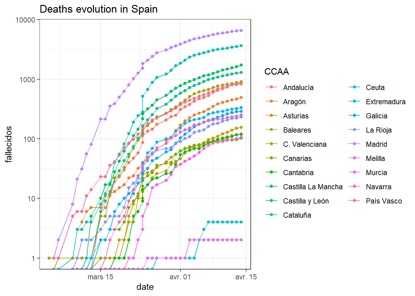
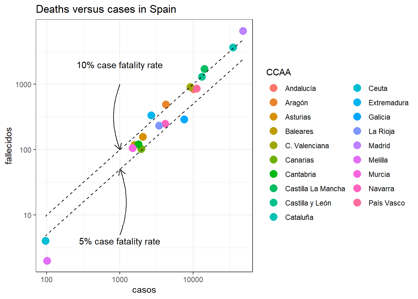
Here a plot comparing the deaths with the confirmed cases in each spanish region:
library(ggplot2)
ggplot(df_tot[date == max(date)])+
  geom_point(aes(casos,fallecidos,color = CCAA),size = 4)+
  geom_line(aes(casos,casos*0.1),linetype = "dashed")+
  geom_line(aes(casos,casos*0.05),linetype = "dashed")+
  theme_bw()+
  scale_y_log10()+
  scale_x_log10()+
  guides(color = guide_legend(ncol = 2))+
  labs(title = "Deaths versus cases in Spain")+
  annotate(geom = "curve",
            x = 1000, y = 1000,
            xend = 1000, yend = 100,
            curvature = .2,
            color="black",
            size = 0.5,
            arrow = arrow(length = unit(3, "mm"))) +
   annotate(geom = "text",
            x = 1000, y = 2000,
            label = "10% case fatality rate",
            hjust = "center",
            color="black")+
    annotate(geom = "curve",
            x = 1000, y = 5,
            xend = 1000, yend = 50,
            curvature = .2,
            color="black",
            size = 0.5,
            arrow = arrow(length = unit(3, "mm"))) +
   annotate(geom = "text",
            x = 1000, y = 4,
            label = "5% case fatality rate",
            hjust = "center",
            color="black")