The comparison function

So, I need to let a bit of variation in my character recognition. There are quite a lot of possibility with the library stringdist, but most of them did not solve the problem I had with the name, which is the following: denis and denisdiego should be the same, but denis and yanis should not. If I try

stringdist("denis","denisdiego")

## [1] 5

stringdist("denis","yanis")

## [1] 2

The distance is greater for the first case, because I need to add 5 characters to go from denis to denisdiego, while I only need to change two characters to switch from denis to yanis. My solution uses the qualV package. Here is the first function I did:

library(qualV)
comp_names <- function(a, b) {
  a <- clean_name(a) # cleaning"
  b <- clean_name(b)
  av <- strsplit(a, '')[[1]] # splitting all characters
  bv <- strsplit(b, '')[[1]] 
  match_str <- paste(qualV::LCS(av, bv)$LCS, collapse='')
  pc <- round(nchar(match_str)/(min(nchar(a), nchar(b)))*100)
  return(pc)
}

I clean the two names a and b, cut it in sequence of character, fin the longest common subsequence, and express it as a percentage of the smallest name. It outputs a similarity on a 100 scale:

comp_names("denis","denisdiego")

## [1] 100

denis and denisdiego are totally similar, while

comp_names("denis","yanis")

## [1] 60

denis and yanis are not so much the same.

Matrix of distances and clustering

I need to calculate the distance between all the entries of a vector, i.e. I need to compute a distance matrix. The distance between two names Tis just 100 - similarity I calculate before. Here is the function to generate the distance matrix:

comp_names_matrix <- function(vec) {
  mat <- sapply(vec, function(x) {
    100 - as.numeric(Vectorize(comp_names)(x, vec))
  })
  rownames(mat) <- vec
  return(mat)
}

comp_names_matrix(df$name)

##               denis denis diego paul sofia sophia, Elèna Paul dénis Paul 
## denis             0           0  100    80            60  100     0   100
## denis diego       0           0  100    60            70  100     0   100
## paul            100         100    0    75            25    0   100     0
## sofia            80          60   75     0            20   75    80    75
## sophia, Elèna    60          70   25    20             0   25    60    25
## Paul            100         100    0    75            25    0   100     0
## dénis             0           0  100    80            60  100     0   100
## Paul            100         100    0    75            25    0   100     0
## Etienne          60          57  100    80            57  100    60   100
## Paule            80          80    0    80            20    0    80     0
## sofia            80          60   75     0            20   75    80    75
##               Etienne Paule sofia
## denis              60    80    80
## denis diego        57    80    60
## paul              100     0    75
## sofia              80    80     0
## sophia, Elèna      57    20    20
## Paul              100     0    75
## dénis              60    80    80
## Paul              100     0    75
## Etienne             0    80    80
## Paule              80     0    80
## sofia              80    80     0

Now I can use the basic tools of clustering to see if I can identify the similar names:

df$name %>%
      comp_names_matrix(.) %>%
      stats::as.dist(.) %>%
      stats::hclust(.) %>% 
  plot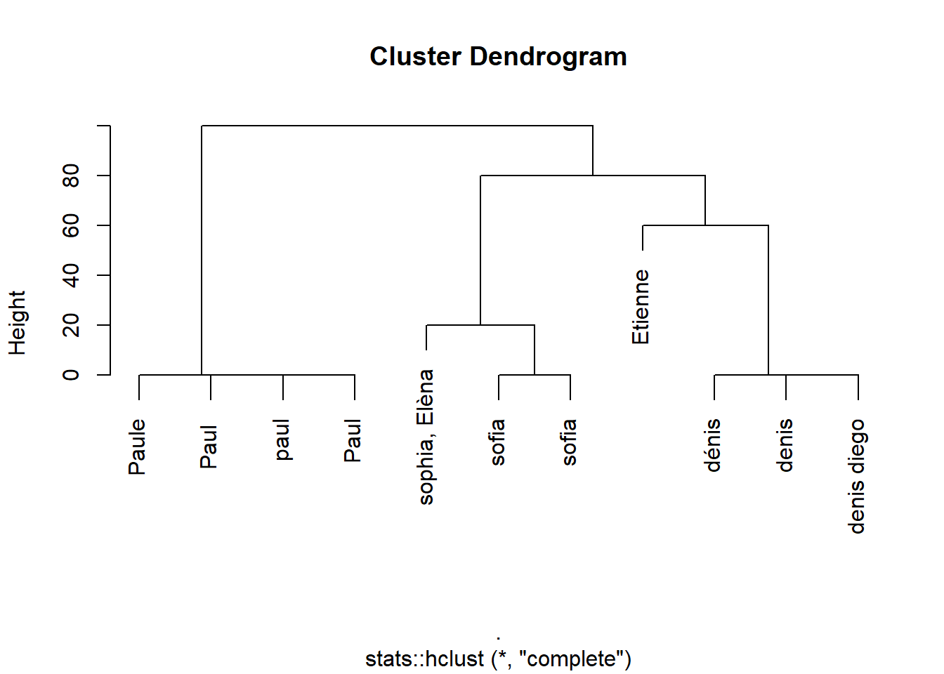 

Here it seems that my distance allow me to detect the similar person in a proper way. I need to find a threshold to produce an index indicating the names that are the same. I see in the dendrogram above that it lies between 20 and 40. The function to use is stats::cutree(h = thres). I write the following, that use the name comparison function described above and detect clusters of names:

compare_tree <- function(vec, thres = 30) {
  if(length(vec)>1){
  output <- vec %>%
    comp_names_matrix(.) %>%
    stats::as.dist(.) %>%
    stats::hclust(.) %>%  # cluster
    stats::cutree(h = thres)}else{output <- as.integer(1)}
  return(output)
}
compare_tree(df$name,30)

##         denis   denis diego          paul         sofia sophia, Elèna 
##             1             1             2             3             3 
##          Paul         dénis         Paul        Etienne         Paule 
##             2             1             2             4             2 
##         sofia 
##             3

It recognize the 4 names.

I can now apply this function on the names, surnames and birthdates too.

df[,name_ind := compare_tree(name,30)]
df[,surname_ind := compare_tree(surname,30)]
df[,birthdate_ind := compare_tree(birthdate,20)]

I define a person index for the common detected name, surname and birthdate:

df[,person := .GRP,by = .(birthdate_ind,surname_ind,name_ind)]

It worked. It is flexible enough to allow small mistakes in birthdate and can handle the fact that sometime there is just one name, sometime there are the 3 names of that same person.

If I do that on my entire COVID19 patient table, my computer turn into that:

I have around 70000 patients, which lead to 4.910^{9} distances to calculate. My solution is nice but cannot be used in a real life situation. I therefore need to constrain the degrees of freedom.

Less degrees of freedom

To avoid calculation of immense distance matrix, I can do grouping operation. What I came up with is to calculate the similarity of the names for person having identical cleaned surname and birthdate:

df[,idx1 := paste0("1_",.GRP,"_",compare_tree(name,30)),
   by = .(birthdate,surname_clean)]

The index is constructed as follow: it starts with 1, then it has the grouping index produced by .GRP, and then the index indicating similar names. This gives me a first index: person with same birthdate and surname, and similar names. I do the same for names and birthdate:

df[,idx2 := paste0("2_",.GRP,"_",compare_tree(surname,30)),
   by = .(name_clean,birthdate)]

and the last one:

df[,idx3 := paste0("3_",.GRP,"_",compare_tree(birthdate,20)),
   by = .(name_clean,surname_clean)]

You see that line 1 and 2 have the same idx1 index: same surname, same birthdate, and similar name detected by my function. You can see also that line 1 and 7 have the same idx3 index: same name, surname, and similar birthdates. I need to somehow reconnect these indices to merge them into one, indicating that the lines 1, 2 and 7 are the same person. The answer came from stack: we need to do graph analysis and identify clusters. We can define the lines as nodes, connected by the 3 indices. Nodes connected are the same person. To do that, I use the igraph library:

df[, rn := .I]
DT <- rbindlist(list(
  df[, .(s=idx1, e=idx2, rn)],
  df[, .(s=idx1, e=idx3, rn)],
  df[, .(s=idx2, e=idx3, rn)]))

df[, rn := .I] just create the row number rn (.I is a shortcut for the row number in data.table, really useful in some complex grouping operation). DT is the list of edges and vertices. Here is the graph:

g <- graph_from_data_frame(DT, directed=FALSE)
print(g)

## IGRAPH ea9b148 UN-- 22 33 -- 
## + attr: name (v/c), rn (e/n)
## + edges from ea9b148 (vertex names):
##  [1] 1_1_1--2_1_1 1_1_1--2_2_1 1_2_1--2_3_1 1_3_1--2_4_1 1_3_1--2_5_1
##  [6] 1_4_1--2_6_1 1_5_1--2_7_1 1_2_1--2_3_1 1_2_2--2_8_1 1_2_1--2_9_1
## [11] 1_3_1--2_4_1 1_1_1--3_1_1 1_1_1--3_2_1 1_2_1--3_3_1 1_3_1--3_4_1
## [16] 1_3_1--3_5_1 1_4_1--3_3_1 1_5_1--3_1_1 1_2_1--3_3_1 1_2_2--3_6_1
## [21] 1_2_1--3_7_1 1_3_1--3_4_1 2_1_1--3_1_1 2_2_1--3_2_1 2_3_1--3_3_1
## [26] 2_4_1--3_4_1 2_5_1--3_5_1 2_6_1--3_3_1 2_7_1--3_1_1 2_3_1--3_3_1
## [31] 2_8_1--3_6_1 2_9_1--3_7_1 2_4_1--3_4_1

I then detect clusters:

cl <- clusters(g)$membership
cl

## 1_1_1 1_2_1 1_3_1 1_4_1 1_5_1 1_2_2 2_1_1 2_2_1 2_3_1 2_4_1 2_5_1 2_6_1 2_7_1 
##     1     2     3     2     1     4     1     1     2     3     3     2     1 
## 2_8_1 2_9_1 3_1_1 3_2_1 3_3_1 3_4_1 3_5_1 3_6_1 3_7_1 
##     4     2     1     1     2     3     3     4     2

DT[, g := cl[s]]

And I merge back the found index in my initial data table, merging on the row number:

df[unique(DT, by="rn"), on=.(rn), person := g]

That’s it !

I put everything in a function: